Survey News Volume 7, Issue 3
Survey News Volume 7, Issue 3
In This Issue:
- 2019 Supplemental Victimization Survey
- Data Collection Underway for the 2019 American Housing Survey
- Response Rate Regression Modeling for the Consumer Expenditure Quarterly Interview Survey
- Internet and Incentive Experiments for the 2018 School Survey on Crime and Safety
- Counties Can Have the Same Median Age But Very Different Population Distributions
- Population Estimates Show Aging Across Race Groups Differs
- Census Bureau Releases First Ever Report on Men’s Fertility
- Other Recent Data Releases
2019 Supplemental Victimization Survey
by Jamie Choi, Survey Statistician, National Crime Victimization Survey Team
Data collection for the 2019 Supplemental Victimization Survey (SVS) started in July. The SVS is a supplement to the National Crime Victimization Survey (NCVS), and both are sponsored by the Bureau of Justice Statistics (BJS). The SVS is designed to measure the prevalence, characteristics, and consequences of nonfatal stalking, and it asks questions related to victims’ experiences of these unwanted contacts or behaviors. The SVS was conducted twice as a supplement to the NCVS from January through June 2006 and July through December 2016. It is administered again from July through December 2019. Respondents ages 16 or over who complete the NCVS are eligible for the SVS.
The SVS begins with a screener instrument asking about each element of the Violence Against Women Act’s (VAWA) definition of stalking. The VAWA, which was amended in 2013, includes elements of presence, actual or reasonable fear, intimidation, emotional distress, and cyberstalking. If a respondent screens in as a stalking victim based on responses to the screener, the survey continues with the incident portion, which focuses on details of the stalking victimization. There are no extensive questionnaire changes for the 2019 SVS.
For more information on stalking and stalking resources, please visit the Stalking Resource Center at //www.victimsofcrime.org/our-programs/stalking-resource-center. For more information about the NCVS from the Bureau of Justice Statistics, please visit
https://www.bjs.gov/index.cfm?ty=dcdetail&iid=245.
Data Collection Underway for the 2019 American Housing Survey
by Tamara Cole, Survey Director, Housing Surveys Team
The American Housing Survey (AHS) collects up-to-date information on housing quality and costs in the United States every two years. The survey is sponsored by the Department of Housing and Urban Development (HUD). The 2019 survey began data collection on June 26.
For 2019, the survey includes supplemental topics on food security, housing accessibility, and post-secondary education:
- Food security was last asked in the 2015 AHS and includes questions regarding the availability and affordability of food.
- Questions regarding housing accessibility and home modifications to assist occupants living with disabilities are based on the 2011 Housing Accessibility supplement, with a new focus on mobility of the respondent and members of their household.
- The post-secondary education topic asks about the current enrollment of household members beyond high school and provides more insight into the educational institution.
Concurrent with the 2019 AHS production data collection, the AHS will conduct a telephone follow-on survey on housing insecurity which will serve as a research vehicle for HUD to study these concepts and as they develop a consistent measure to track the prevalence of housing security over time. They will also use information collected from the follow-on survey in correlation with housing and other topics like health, education, and employment. The sample for the follow-on survey is comprised of 4,000 respondents who meet certain criteria based on their responses to the 2019 AHS CAPI production questionnaire.
Over 3,000 new field representatives have been hired to work on the AHS this summer. We expect to closeout data collection in October and publish results in the summer of 2020.
Response Rate Regression Modeling for the Consumer Expenditure Quarterly Interview Survey
by John Gloster, Assistant Survey Director, Consumer Expenditure Survey Team
The Consumer Expenditure Surveys (CE) is a household survey program sponsored by the U.S. Bureau of Labor Statistics. Survey data is collected by the U.S. Census Bureau and has seen an average national response rate of 74.8% for the CE Quarterly Interview Survey (CEQ) in FY2009 steadily drop to an average of 58.5% by 2018. This trend has continued into FY2019 with CEQ response rates averaging 55.2% nationwide (as of the June 2019 closeout). In a continuing effort to combat survey nonresponse, we designed a Response Rate Regression (R3) model for the CE by making use of various interviewer and caseload attributes. Differing from other survey management techniques such as adaptive design, this R3 modeling focuses on key variables and survey attributes whose values are prescribed prior to data collection and carried through until the end of the survey cycle. The R3 modeling serves to help identify specific areas where survey management, logistics, and data collection protocols can improve. This is accomplished by isolating variables of significance to determine the degree by which these variables (or programmatic aspects) affect survey response rates.
The first step in developing the CEQ R3 model was to extract 2018 production data for CEQ within the Regional Office Survey Control system using SQL code. The second step in developing the model involved extracting data from a CEQ Field Representative (FR) Training Enhancement Survey. This survey was issued to all CEQ field staff nationwide, and was fielded by the Field Financial Surveys Branch from April 1, 2019 through April 14, 2019 via Survey Monkey. The survey allowed for the collection of notable information at the FR level, which was integral for incorporation into the CEQ R3 model. These data included tenure, presence of a second job, personality associations, Spanish language proficiency, prior interviewing experience, educational attainment, multiple survey workloads, etc. The third step in model development was the merging and refining of the two datasets to prepare the final dataset for integration into a SAS regression procedure. The final dataset resulted in the creation of fourteen predictor variables and one intercept variable for the CEQ R3 model.
A SAS stepwise regression technique with a confidence interval of 0.95 was used to analyze the model dataset, which consisted of 379 observations across all six Regional Offices. Holding all else constant, the CEQ R3 model has shown that the most significant indicators of interviewer success are:
1. the number of new Wave 1 cases assigned to the interviewer,
2. whether or not the interviewer has another job outside of the Census Bureau field representative position, and
3. the total number of other surveys concurrently worked by the interviewer.
However, these results are based on a finite dataset that does not account for the other countless number of interviewer, programmatic, and respondent-driven variables existing within the CEQ survey paradigm, and the resulting response rate model is purely the product of a limited input.
Using regression to predict a survey’s response rate can provide more statistical power and a stronger basis for inference as opposed to the sole use of base frequencies and statistical averages. The R3 model allows an analyst to obtain a more complete picture in terms of how various aspects of data collection correlate with one another, and to provide a more complete story regarding a program’s response rate trends.
Internet and Incentive Experiments for the 2018 School Survey on Crime and Safety
by Tracae McClure, Survey Statistician, Education Surveys Team
The School Survey on Crime and Safety (SSOCS) is sponsored by the National Center for Education Statistics (NCES) within the U.S. Department of Education. It was first conducted in 2000 and in the following subsequent years: 2004, 2006, 2008, 2010, and 2016. Since 2006, NCES entered into recurring interagency agreements with the U.S. Census Bureau’s Education Surveys Team in the Demographic directorate to conduct the SSOCS.
The SSOCS collects detailed information on the incidence, frequency, seriousness, and nature of violence affecting students and school personnel, as well as other indicators of school safety from the schools’ perspective.
Traditionally, SSOCS is a multi-mode survey, mainly conducted by mail, with telephone and e-mail follow-up. The SSOCS 2018 included two data collection experiments:
1. testing the inclusion of an internet instrument as a mode of completing the survey; and
2. testing the inclusion of a $10 cash incentive for respondents.
Both experiments were added with the goal of increasing response rates and decreasing time to complete the survey.
These two experiments were implemented in a factorial design to study the main effects of each intervention and any interaction between the two experiments. Schools were randomly assigned to the internet and incentive treatments at the time of sampling. The design of the experiments is presented below.
|
Internet |
|||
Yes |
No |
Total |
||
Incentive |
Yes ($10) |
575 |
1,825 |
2,400 |
No ($0) |
575 |
1,825 |
2,400 |
|
Total |
1,150 |
3,650 |
4,800 |
|
Schools in the internet group had the option to respond online via a web-first strategy where the first two mailings provided a URL and login information, and the final two mailings provided a paper questionnaire. The control group received a paper questionnaire throughout data collection and did not receive the option to respond online[1]. The web instrument was developed by Centurion programmers. Items on the web instrument were presented in the same order to reflect the paper questionnaire. In addition, definitions or words embedded within questions were presented to respondents via pop-ups.
Data collection started in February 2018 and concluded in June 2018. Follow-up telephone operations were conducted using the Jeffersonville Contact Center throughout the later portion of data collection.
This article highlights the key findings of three analyses projects conducted by the Demographic Statistical Methods Division (DSMD) on the multi-mode experiment included in SSOCS 2018. These key findings include the (1) effect of data collection analysis, (2) paradata analysis, and (3) analysis of the internet/incentive experiments.
1. Effect of Data Collection Methodology
DSMD evaluated the effect of the data collection methodologies (paper with telephone follow up vs. web with paper and telephone follow up) offered for SSOCS 2018. Results indicated an overall response rate of 60.2%[2], with the paper treatment response rate of 60.1% and the web treatment response rate of 60.2%. Among school characteristics, only a significant difference was found among the treatment groups for the student to full-time equivalent teaching staff ratio. When looking at selected item completion rates, item responses from the web instrument were nominally higher but lower for follow-up items. However, the web instrument showed no impact when evaluating selected key estimates.
2. Paradata
DSMD analyzed respondent interactions on the web survey instrument. Paradata were captured from the following interactions: device use, logins, lag time between logins, completion times, breakoffs, changed answers, errors rendered, previous clicks, links clicked, and questionnaire downloads.
Of the 1,150 sub-sample of respondents offered the web instrument, 758 respondents accessed the instrument. The majority of respondents (99.1%) who accessed the instrument, completed it on a computer instead of a smartphone or tablet. Sixty percent of respondents who completed the survey did so in one session or logged in only one time. The median response time was approximately 29 minutes for respondents to complete the survey online in one session in comparison to an average 55 minutes when completing the paper questionnaire (as reported by paper questionnaire respondents).
The page with the highest number (42.1%) of breakoffs was the Assign_pin page. This page appears after the respondent enters their User ID on the log in page, provides the respondent a 4-digit pin, and asks the respondent to select and answer a security question. To investigate this further, DSMD will be conducting similar analyses across all of the NCES-sponsored Education Surveys projects.
3. Internet Incentive Experiments
When investigating the response rates of the various treatment groups compared to the control group, results showed a significant difference in the response rates of schools who received an incentive but no option to respond online when compared to schools who did not receive an incentive or internet response option (control group). Although not statistically significant, schools who received an incentive and the option to respond online had a higher response rate than the control group.
Approximately eighty-eight percent of schools assigned to the internet treatment group responded online. When assessing response times, results indicated the incentive, regardless of the internet option, produced the fastest response time. All treatment groups observed significantly faster response time compared to the control group.
When assessing whether offering a $10 cash incentive impacted the breakoff rate for respondents who completed the survey online, results showed schools in the internet treatment group that did not receive an incentive had a weighted breakoff rate of 11.7 percent, compared to those that did receive an incentive at 10.3 percent; however, the analysis did not provide evidence that the incentive influenced the breakoff rate among those who used the web.
Overall, the analysis indicated incentives led to an increase in response rates. Being in the web treatment group alone did not increase response rates, but it also did not induce nonresponse bias. Further, respondents appeared to prefer the web response option.
Based on the results from these analyses, the following methodological changes will be made for the SSOCS 2020 collection:
- Data will be collected primarily by web, with paper questionnaires included in the third and fourth mailed packages to nonresponding schools.
- Pages with high breakoff rates will be reorganized and split into separate pages to reduce response time and improve readability.
- Incentives will continue to be provided, but there are plans to test a delayed offering to entice nonrespondents at a later mailing.
- A navigation menu is being tested to improve instrument usability and/or reduce respondent burden.
To learn more about SSOCS, the analyses, and references supporting the analysis conducted by the Demographic Statistical Methods Division, contact Tracae McClure at [email protected].
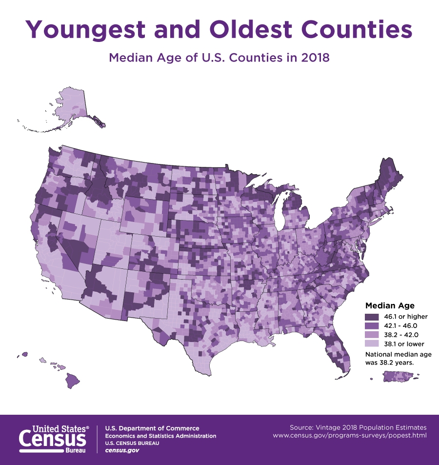
Counties Can Have the Same Median Age But Very Different Population Distributions
by Luke Rogers, Branch Chief, Population Estimates Branch, Population Division
The nation’s median age was 38.2 in 2018, up from 37.2 in 2010, but new county population characteristics released by the U.S. Census Bureau on June 20, 2019, show that age is more than a number.
Two or more counties can have the same median age — the point when half the population is older and half younger — yet have age profiles of their populations that are completely different.
Some may have relatively large shares of young adults and not many children or older people while other counties can have large proportions of children and 35- to 59-year-olds (i.e., their parents). Despite these compositional differences, these counties can have roughly the same median age.
To illustrate this, let’s look at three counties that have roughly the same median age as the nation and as each other.
Same Median Age, Different Age Structures
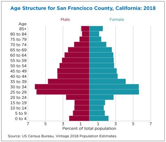
California’s San Francisco County — which has the same boundary as the city of San Francisco — had a median age of 38.2 in 2018, a slight decrease from 38.5 in 2010.
San Francisco County is home to many 25- to 39-year-olds who collectively make up almost a third (32.5%) of the total county population. The “population pyramid” below shows how the size of the county’s age groups, broken down by sex, is distributed.
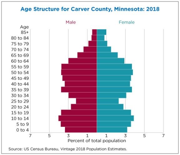
Now compare San Francisco County with Carver County, Minnesota, which is a part of the Minneapolis-St. Paul-Bloomington, MN-WI metropolitan area.
In 2018, Carver County’s median age was 38.1, up from 36.3 in 2010. The age structure in Carver County has two distinct groups: those under the age of 20 and those ages 35 to 59 — basically children and the parents of those children.
Carver County has about the same median age as San Francisco County, but its age structure is almost the inverse. One has a large population of children and 35- to 59-year-olds (Carver) while the other has a lot of 25- to 39-year-olds (San Francisco).
When No Age Group Dominates
Some counties have no one age group that sticks out.
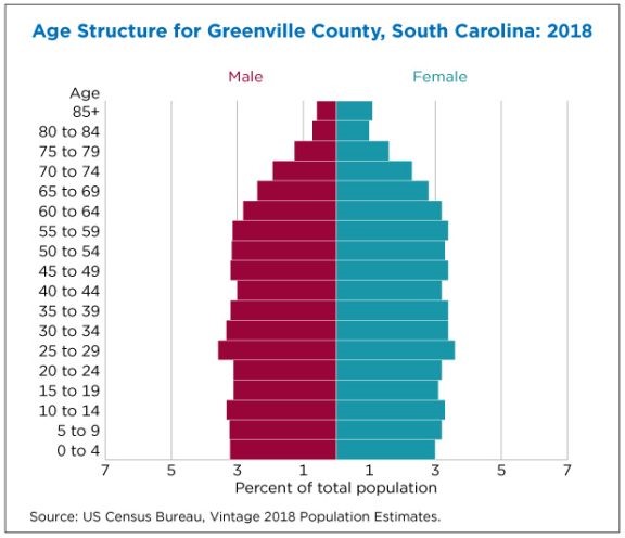
For example, Greenville County in South Carolina, part of the Greenville-Anderson-Mauldin, SC metropolitan area, had a median age of 38.2, up from 37.2 in 2010.
Greenville County’s median ages in 2010 and 2018 were the same as the nation’s, and its age structure is very similar to the nation’s as well. The population is more evenly distributed across most age groups, unlike the distinct age groups that dominate in San Francisco County and Carver County.
Median age is useful in summarizing whether a population is aging, but it’s important to remember that there is more to the age structure of the population than the snapshot that median age alone can provide.
Population Estimates Show Aging Across Race Groups Differs
by Jewel Jordan, Public Affairs Specialist, Media Relations Branch, Public Information Office
North Dakota Only State to Get Younger
The nation as a whole continues to grow older with the median age increasing to 38.2 years in 2018, up from 37.2 years in 2010. The pace of this aging is different across race and ethnicity groups, according to new 2018 Population Estimates by demographic characteristics for the nation, states and counties, released June 20, 2019 by the U.S. Census Bureau.
From 2010 to 2018, the U.S. population’s median age increased by 1.0 years. Amongst the different race groups:
- The white alone-or-in-combination population increased by 1.0 years.
- The black or African American alone-or-in-combination population grew by 1.4 years.
- The American Indian and Alaska Native alone-or-in-combination population increased by 2.2 years.
- The Asian alone-or-in-combination population increased by 1.7 years.
- The Native Hawaiian and Other Pacific Islander alone-or-in-combination population increased by 2.6 years.
- The Hispanic (any race) population experienced an increase in median age of 2.2 years.
"The nation is aging — more than 4 out of every 5 counties were older in 2018 than in 2010. This aging is driven in large part by baby boomers crossing over the 65-year-old mark. Now, half of the U.S. population is over the age of 38.2," said Luke Rogers, the Chief of the Population Estimates Branch at the Census Bureau. "Along with this general aging trend, we also see variation among race and ethnicity groups both in growth patterns and aging." Rogers also noted that alone-or-in-combination groups overlap and individuals who identify as being two or more races are included in more than one of these race groups.
At the state level, North Dakota was the only state to see a decline in its median age, from 37.0 years in 2010 to 35.2 in 2018. Maine had the largest increase in median age this decade, going from 42.7 years in 2010 to 44.9 years in 2018, making it the state with the highest median age in the country. Utah had the lowest median age in 2018, at 31.0 years.
The share of the population age 65-and-older was 16.0 percent in 2018, growing by 3.2 percent (1,637,270) in the last year. The 65-and-older age group has increased 30.2 percent (12,159,974) since 2010. In contrast, during the same period, the under 18 population decreased by 1.1 percent, or a decline of 782,937 people.
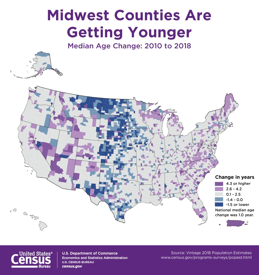
Of the nation’s 3,142 counties, 2,566 (81.7 percent) had a higher median age in 2018 than in 2010. During this period, 16.7 percent (525) had median age decreases and 1.6 percent (51) saw no change. In 2018, out of all counties, 56.2 percent (1,767) had a median age between 40 and 49 years. Among those counties with populations of 20,000 or more in 2017 and 2018, Sumter County, Florida, had the highest median age (67.8) and Madison County, Idaho, had the lowest median age (23.2).
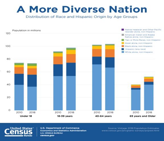
A Changing Nation
As the nation continues to grow older, it is also changing by race and ethnicity. View our graphic on the age and race distribution from 2010 to 2018 to see how the nation has grown more diverse. References below to the race and ethnicity compositions are for race-alone-or-in-combination groups or Hispanic (any race) unless otherwise specified.
- Of the 50 states and the District of Columbia, 20 had a white population of 5.0 million or more, 21 were between 1.0 million and 4.9 million, nine were between 500,000 and 999,999, and one, the District of Columbia, had a population between 100,000 and 499,999.
- In 2018, 18 states had a black population greater than or equal to 1.0 million.
- California was the only state to have an Asian population larger than 5 million, at 6,890,703 in 2018. New York (1,922,974) and Texas (1,688,966) were the only two states that had a population between 1.0 million and 4.9 million.
- The American Indian and Alaska Native population was over 1.0 million in only one state, California, at 1,089,694 in 2018.
- In 2018, 36 states and the District of Columbia had a Native Hawaiian and Other Pacific Islander population that was less than 20,000. The two states with the largest Native Hawaiian and Other Pacific Islander populations in 2018 were Hawaii (382,261) and California (363,437).
- In 2018, the Hispanic population was between 100,000 and 499,999 in 20 states. Among the states and the District of Columbia, 10 states had a Hispanic population of 1.0 million or more. California (15,540,142), Texas (11,368,849), and Florida (5,562,417) were the only states that had populations of 5.0 million or more.
The Hispanic Population (of any race)
- Hispanic population in the United States grew by 2.0 percent (1,164,289) between 2017 and 2018.
- In 2018, the Hispanic population was greater than or equal to 50,000 in 5.6 percent (177) of counties and less than 100 people in 5.5 percent (173) of counties. Of counties with populations of 20,000 or more in 2017 and 2018, the Hispanic population had the fastest growth in Liberty County, Texas, increasing by 11.4 percent (2,369).
- The Hispanic population was the largest in Los Angeles County, California, with a population of 4.9 million in 2018. The largest numeric growth between 2017 and 2018 was in Maricopa County, Arizona, increasing by 34,395 (2.6 percent) people.
The Black or African American Population
- In 2018, 740 of the 3,142 counties (23.6 percent) had a black or African American population between 1,000 and 4,999 people and 24.1 percent (756) of counties had a black or African American population between 100 and 499 people.
- Cook County, Illinois, had the largest black or African American population, which was about 1.3 million in 2018. Harris County, Texas had the largest numeric increase between 2017 and 2018, gaining 14,017 (1.5 percent) people.
- Of counties with a total population of 20,000 or more in 2017 and 2018, the black or African American population had the fastest increase in Ellis County, Texas, growing by 9.0 percent (1,799) between 2017 and 2018.
The Asian Population
- In 2018, 2.7 percent (86) of counties had an Asian population of 50,000 people or more. The Asian population was less than 1,000 people in 73.1 percent (2,297) of counties.
- Los Angeles County, California, had the largest Asian population in 2018 (1,720,889). King County, Washington, had the largest numeric increase in the Asian population, increasing by 23,932 (5.1 percent) between 2017 and 2018.
- Among counties with a total population of 20,000 or more in 2017 and 2018, the Asian population grew the fastest in Forsyth County, Georgia, increasing by 11.5 percent (3,734) between 2017 and 2018.
The American Indian and Alaska Native Population
- In 2018, 20 counties (0.6 percent) had an American Indian and Alaska Native population of 50,000 or more. Also in 2018, 635 counties (20.2 percent) had an American Indian and Alaska Native population between 1,000 and 4,999 and 1,272 (40.5 percent) counties had an American Indian and Alaska Native population that was between 100 and 499. The American Indian and Alaska Native population was less than 1,000 people in 2,219 (70.6 percent) counties.
- Los Angeles County, California had the largest American Indian and Alaska Native population in 2018 (231,340). Maricopa County, Arizona, had the largest numeric increase, growing by 3,745 (2.4 percent).
- Among counties with a total population of 20,000 or more in 2017 and 2018, the American Indian and Alaska Native population had the fastest growth in Clark County, Nevada, increasing by 3.5 percent (1,690) between 2017 and 2018.
The Native Hawaiian and Other Pacific Islander Population
- In 2018, only three (0.1 percent) counties had a Native Hawaiian and Other Pacific Islander population of 50,000 or more — these were Honolulu County (245,043) and Hawaii County (70,910) in Hawaii, and Los Angeles County, California (67,730). In 2018, 578 (18.4 percent) counties had a population between 100 and 499 people and 2,217 (70.6 percent) counties had a Native Hawaiian and Other Pacific Islander population that was less than 100 people.
- Honolulu County, Hawaii, had the largest Native Hawaiian and Other Pacific Islander population at 245,043 people in 2018. Clark County, Nevada, had the largest numeric growth, increasing by 1,458 between 2017 and 2018.
- Among counties with a population of 20,000 or more in 2017 and 2018, Pierce County, Washington, had the fastest Native Hawaiian and Other Pacific Islander population increase, growing by 4.9 percent (1,085) between 2017 and 2018.
The White Population
- The white population remained the largest group in the nation at 78.9 percent (258,080,572), and had the largest numeric increase from 2017 to 2018 (1,055,588).
- In 2018, the white population was greater than or equal to 50,000 in 906 (28.8 percent) counties and between 10,000 and 49,999 people in 1,390 (44.2 percent) of counties. In 2018, 48 (1.5 percent) counties had a white population that was less than 1,000 people.
- Los Angeles County, California, had the largest white population, at 7.4 million in 2018. Maricopa County, Arizona had the largest increase in the white population between 2017 and 2018, growing by 60,749 (1.6 percent).
- Among counties with a population of 20,000 or more in 2017 and 2018, Williams County, North Dakota, had the fastest growth in the white population at 5.3 percent (1,596) between 2017 and 2018.
For additional information about population changes by age and for each race or ethnic group, view our detailed tables. This is the last release of the population estimates for 2018. Previous estimates included national, county, metro area, city and town population estimates. These estimates are as of July 1, 2018, and therefore do not reflect the effects of Hurricane Florence in September 2018, Hurricane Michael in October 2018, and the California Wildfires. For information on how the national population is projected to change through 2060, view our previous release, Older People Projected to Outnumber Children for First Time in U.S. History.
Unless otherwise specified, the statistics refer to the population who reported a race alone or in combination with one or more races. Censuses and surveys permit respondents to select more than one race; consequently, people may be one race or a combination of races. The detailed tables show statistics for the resident population by "race alone" and "race alone-or-in-combination." The sum of the populations for the five "race alone-or-in-combination" groups adds to more than the total population because individuals may report more than one race. The federal government treats Hispanic origin and race as separate and distinct concepts. In surveys and censuses, separate questions are asked on Hispanic origin and race. The question on Hispanic origin asks respondents if they are of Hispanic, Latino or Spanish origin.
Starting with the 2000 Census, the question on race asked respondents to report the race or races they consider themselves to be. Hispanics may be of any race. Responses of "some Other Race" from the 2010 Census are modified in these estimates. This results in differences between the population for specific race categories for the modified 2010 Census population versus those in the 2010 Census data.
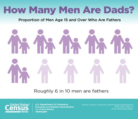
Census Bureau Releases First Ever Report on Men’s Fertility
by Jewel Jordan, Public Affairs Specialist, Media Relations Branch, Public Information Office
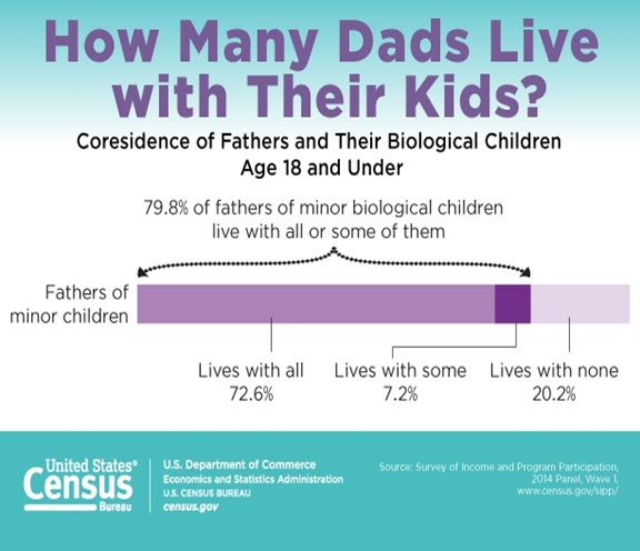
About 61.6% of men (74.7 million men) age 15 and over are fathers, and of those, 72.2 million men have a biological child, according to a new Men’s Fertility and Fatherhood: 2014 report released on June 13, 2019 by the U.S. Census Bureau. More than one in four men have a biological child under the age of 18. Of the men with biological children under age 18, four out of five live with at least some of those minor children.
The report comes from the 2014 Survey of Income and Program Participation (SIPP), which is the first Census Bureau survey to ask about the full fertility histories for both men and women.
This report shows the diversity of men’s fatherhood experiences and examines the relationships between men and the children with whom they live, including their own and their partners’ children, and how those relationships are related to other aspects of men’s lives.
“For the first time, we’re able to look at the fertility of men as well as women,” said Lindsay Monte, a demographer in the Fertility and Family Statistics Branch at the Census Bureau. “When looking at the full fertility histories of men, we see a depth and complexity to the experiences of fatherhood that we have not been able to see before in our data.”
Over one-third of men are married and have biological children with their spouse. There are also 2.9 million men (2.4%) who are living with an unmarried partner and have biological children with that partner. Nearly one in ten men have children with more than one person.
“While most fathers live with at least some of their biological children, they also live with a variety of other children,” said Monte.
“About 4 million men live with 5.6 million minor stepchildren or other children of an unmarried partner.”
Additionally, about 13 million men live with about 23 million other children ages 0 to 17, including grandchildren, nieces or nephews, minor siblings, and foster children. There are 29.2 million grandfathers, or roughly 24.1% of all men age 15 and over. Of the men who live with their own, or a spouse or partner’s children under age 18, about 1% also live with grandchildren.
The report also gives an in-depth look at the demographics of fatherhood.
Relationships
- Of the 72.2 million fathers, 5.9 million (8.2%) have never been married.
- About 73.4% of fathers are married, 12.9% are divorced, 3.2% are widowed, and 2.3% are separated.
Race
- About 1% of white, Asian and Hispanic men ages 15 to 19 are fathers, compared with about 3% of black men of the same age.
- Among men ages 20 to 29, 21.2% of white men, 24.9% of black men, 12.4% of Asian men, and 29.4% of Hispanic men are fathers.
Educational Attainment
- About 14% of fathers do not have a high school diploma, and roughly 12% of fathers hold a graduate or professional degree.
- Among men ages 40 to 50 years, men with a bachelor’s degree are less likely to have children than men with less than a high school diploma.
Fathering
“The experience of being a father isn’t just limited to the number of children men have, but includes the act of fathering their children,” Monte said. “Research has found that parents eating dinner with their children is associated with a range of benefits for children, including expanded vocabulary, fewer behavior problems, and lower likelihood of substance abuse among teenagers.”
Roughly three-quarters of men who live with biological or adopted children under age 18 eat dinner with those children between five and seven nights per week, regardless of the age of the children. Outings with children are also associated with positive child development and are an indicator of parental involvement. Around 40% of men in all family types take young children on outings at least three times a week.
To learn more about the marital status of fathers and the relationships between men and their partners’ minor children, visit America Counts: Stories Behind the Numbers.
The SIPP is a nationally representative panel survey administered by the Census Bureau that collects information on the short-term dynamics of employment, income, household composition, and eligibility and participation in government assistance programs. Each SIPP panel follows individuals for several years, providing monthly data that measure changes in household and family composition and economic circumstances over time.
Other Recent Data Releases
June 2019 Releases
Nonemployer Businesses Increased in 2017- The number of nonemployer businesses — establishments without paid employees — grew 3.6% from 24,813,048 to 25,701,671 in 2017, according to U.S. Census Bureau statistics released on June 27. Receipts for these businesses increased 5.6%, adding more than $65.7 billion from 2016 to 2017 (June 27).
May 2019 Releases
2014 Survey of Income and Program Participation Multiple Jobholders Report- The U.S. Census Bureau released the Multiple Jobholders Report. This report uses data from the 2014 Survey of Income and Program Participation (SIPP) to examine the characteristics of people who held multiple jobs in 2013. The report looks at jobholders by sex, industry, occupation and work schedule. In addition, the analysis includes seasonality of multiple jobholding (May 29).
Fastest-Growing Cities Primarily in the South and West- The South and West continue to have the fastest-growing cities in the United States, according to new population estimates for cities and towns released May 23 by the U.S. Census Bureau. Among the 15 cities or towns with the largest numeric gains between 2017 and 2018, eight were in the South, six were in the West, and one was in the Midwest (May 23).
U.S. School Spending Per Pupil Increased for Fifth Consecutive Year, U.S. Census Bureau Reports- The amount spent per pupil for public elementary and secondary education (prekindergarten through 12th grade) for all 50 states and the District of Columbia increased by 3.7% to $12,201 per pupil during the 2017 fiscal year, compared to $11,763 per pupil in 2016, according to new tables released May 21 by the U.S. Census Bureau (May 21).