Case Study: Simple MA
Case Study: Simple MA
The U.S. Census Bureau is a world leader in seasonal adjustment research and time series software. This case study is part of a series to keep data users informed of research and encourage discussion. The views expressed on statistical issues are those of the author and not those of the Census Bureau. Displayed code, which is used togenerate plots and figures, is written in the R language.
Moving Average Filters
A linear filter maps an input time series {Xt} to an output time series {Yt} by taking a linear combination of past, present, and future observations:

The filter coefficients (or filter weights) are {ψk}. Note the convention that ψk weights an observation occuring k time points in the past (viewing time t as the present).
Simple Moving Average
In nonparametric regression we may estimate a slowly-changing mean via averaging over neighboring values, e.g.,

This weights the past m and the future m observations equally, and is an example of a linear filter. It also called a moving average, because the observations are averaged (over a window of 2m + 1 time points) in a way that moves over the time series. A simple moving average has equal weights (a general moving average could have unequal weights).
Example: Smoothers Applied to Gasoline Sales
- Linear filters that suppress oscillations and reveal long-term trends are called smoothers. A simple moving average is an example of a smoother.
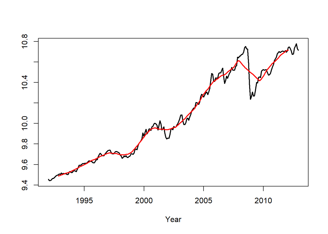
- We apply a simple moving average with m = 10 to the logged seasonally adjusted gasoline series.
gassa <- read.table("GasSA_2-11-13.dat")
gassa.log <- ts(log(gassa),start=1992,frequency=12)
h <- 10
simple.ma <- rep(1,2*h+1)/(2*h+1)
gas.trend <- filter(gassa.log,simple.ma,method="convolution",sides=2)
gas.trend <- ts(gas.trend,start=1992,frequency=12)
plot(ts(gassa.log,start=1992,frequency=12),col=1,ylab="",xlab="Year",lwd=2)
lines(ts(gas.trend,start=1992,frequency=12),col=2,lwd=2)

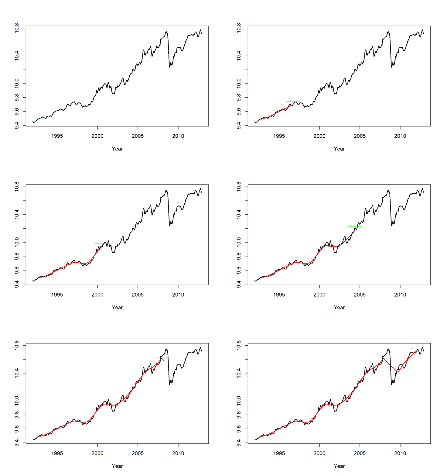
- We want to express this action as a movie.
flex <- 0
siglen <- length(gas.trend) - 2*h
range <- seq(1,siglen,1)
for(t in range)
{
filterweight <- c(rep(NA,t-1),simple.ma + gas.trend[h+t] + flex,
rep(NA,siglen-t))
plot(ts(gassa.log,start=1992,frequency=12),col=1,ylab="",xlab="Year",lwd=2)
lines(ts(gas.trend[1:(h+t)],start=1992,frequency=12),col=2,lwd=2)
lines(ts(filterweight,start=1992,frequency=12),col="#00FF0090",lwd=2)
}


