The U.S. Census Bureau is a world leader in seasonal adjustment research and time series software. This case study is part of a series to keep data users informed of research and encourage discussion. The views expressed on statistical issues are those of the author and not those of the Census Bureau. Displayed code, which is used to generate plots and figures, is written in the R language.

Bandpass filters are routinely used by economists, statisticians, and others to extract out the cyclical component of a time series related to the business cycle. The sequences of expansions and contractions in economic conditions, related to business cycle for the macroeconomy, typically have a range of periods such as 2 to 10 years. These phases can have substantial effects on the welfare of the United States’ population and on policy decisions of major government institutions. In this entry we describe a more reliable and modernized band-pass filter methodology. It is well-known that different macroeconomic time series, e.g. Consumption of Services and Residential Investment (for both, the source is the Bureau of Economic Analysis; in Trimbur and McElroy (2022+), quarterly data from 1947:1 to 2019:4 is used), their respective cyclical movements over the aggregate business cycle can differ considerably. It is less well-known how to quantitatively measure such differences in a valid and statistically sound manner, a question I have striven to answer decisively in our research in this field.

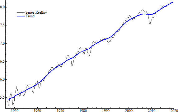
Let’s examine a particular measure of economic activity. Figure 1 shows data for Real Investment (Source: Bureau of Economic Analysis) from the first quarter of 1947 to the last quarter of 2019. The black dotted line represents the data (displayed in logarithms). One can see how, over long intervals such as twenty year periods, the Investment time series tends to rise. The solid blue line indicates a trend line that reflects such rises and is produced by applying a filter, which essentially just weights each observation by a certain amount and sums all the terms together. Many such filters are possible. In Figure 1 the trend is produced using a statistical model, a method that establishes the filter and trend in an econometrically coherent manner; this provides significant advancements over previous approaches, as discussed below.

In Figure 1 it can also be seen that there are persistent movements in the original time series around the trend, representing times of general expansion relative to trend as well as times of weaker performance compared to trend. These boom-bust sequences reflect how business cycle fluctuations specifically manifest in a given time series, such as the Investment data investigated here. The aim of a band-pass filter is then to clarify the cyclical movements by removing the trend and any residual noise due to factors like measurement error.

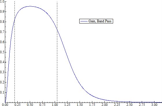
Band-pass filters are naturally defined in the frequency domain, which is the dual aspect of the time domain, which concentrates on correlations and movements over time. In contrast the frequency domain expresses data fluctuations in terms of the kinds of cycles it contains, and it provides the sophisticated and flexible treatment of periodicity (e.g., it incorporates variation in amplitudes and phases) needed in the analysis of economic cycles. Two examples of band-passes are indicated in Figure 2; the black dotted line (with a segment at 1.0 connecting the two vertical ones) represents the “ideal” filter, so called in earlier work like Baxter and King (1999) because it completely blocks out frequency parts outside a chosen band. Here, we will depart from what was previously conventional usage and adopt the terminology “block” filter rather than “ideal” filter (as used in the previous work of Baxter and King (1999). Our revised nomenclature proposes a more accurate portrayal of band-pass filters as applied to economic data and is designed to help steer the researcher and other users away from the false notion that the block filter would be one’s first choice in all situations, such as in fields outside of engineering.

In Figure 2, it is clear that the blue curve is based on a more flexible concept where a band-pass filter has a general tendency for selecting mid-range frequencies, without having to be perfectly sharp like the block filter. The specific shape taken by the flexible band pass filter is generated from a basic statistical/econometric decomposition model. This expresses the series of interest as a sum of stochastic trend, cyclical part, and noise. With the model fitted and tailored to the data, we use the terminology “adaptive” band-pass for the particular filter that provides the best cycle estimator. The precise selection of the blue band-pass in Figure 2 and more generally of the adaptive filter for any given time series is chosen to minimize the average error in the extraction of the cyclical part in the stochastic setup. Hence the band-pass adapts to the dynamic properties of the series at hand.

The extracted cycle in Investment, yielded by the adaptive band-pass in Figure 2, is displayed in Figure 3. There one can note immediately the changing separation between subsequent peaks, for instance, and the time variation in the span, or amplitude, of the fluctuations. An approximation to the block filter such as the Baxter-King (BK) filter would give a different extracted cycle, corresponding to the different gain functions. Here we keep the treatment concise and give a different illustration that highlights the divergences in the two filters.

Figure 4 shows a simulated series of simple white noise observations as the green dotted line. The trend, indicated by the solid blue line, is basically flat. This kind of series could represent say, successive increments in a stock price in the financial markets, perhaps at a relatively short horizon such days or months.

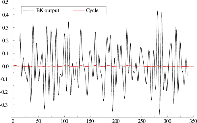
Now Figure 5 gives the BK output as the black dotted line, which appears to indicate an erratic and rapid sequence of peaks and troughs of varying amplitude and duration. Such a result indicating correlations and patterns in white noise appears misleading; when used in financial econometrics it could imply a false interpretation of cyclicality and predictability in stock price changes.

Now, on the other hand, in the adaptive strategy we estimate a statistical model that includes a cyclical component (representing the manifestation of business cycle fluctuations) and the major trend and noise components that may also play a role in a series’ overall movements. The output from the associated model-based filter is indicated by the red line in Figure 5. The difference between the two results is striking in how the modelled approach yields an essentially non-existent cycle (such lack of predictability seems more consistent with the financial economics literature on the analysis of stock returns).

References

- Baxter, M. and King, R.G., 1999. Measuring business cycles: approximate band-pass filters for economic time series. Review of economics and statistics, 81(4), pp.575-593.
- Trimbur, T. and McElroy, T., 2022+. Modelled approximations to the ideal filter with application to time series of Gross Domestic Product. Forthcoming, The Annals of Applied Statistics.