The U.S. Census Bureau is a world leader in seasonal adjustment research and time series software. This case study is part of a series to keep data users informed of research and encourage discussion. The views expressed on statistical issues are those of the author and not those of the Census Bureau. Displayed code, which is used to generate plots and figures, is written in the R language.

AR(1) filter

A simple yet impactful model in time series analysis is the autoregressive model of order 1. It has the representation

for a white noise sequence {wt}. For the sake of this blog we will restrict our attention to the causal AR(1) model specification. This essentially says we will only consider values of ϕ < 1. The topic when ϕ > 1 would be a good one for another blog.

In practice, we get to observe a sample path of the process Xt. A sample path generated from Equation (1) can visually look very difference depending on the value of ϕ. This is in part due to the fact the autocovariance function (ACF) of an AR(1) is given by

for h ∈ {0,±1,±2, . . .}.

One of my favorite ways to visualize this is to consider the white noise sequence of the AR(1) recursion to be fixed; then view sample paths generated for different values of ϕ.

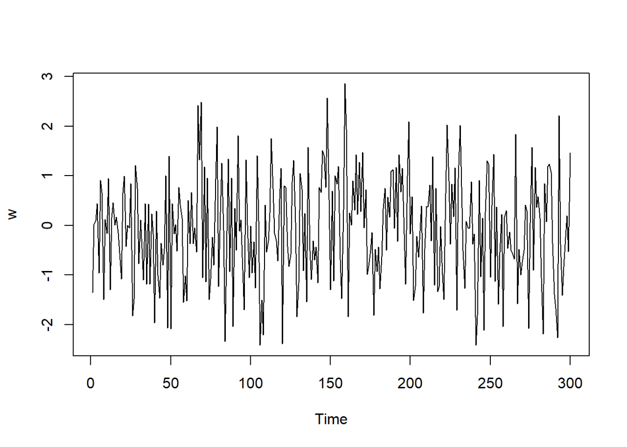
For sample size 300, this will be our white noise sequence.

n = 300
w = rnorm(n)
plot.ts(w)

For a very small value of ϕ, say ϕ = 0.1 the plot of white noise and the AR(1) model are aesthetically similar.

x = arima.sim(list(ar = .1), n = n, innov = w)
plot.ts(x)

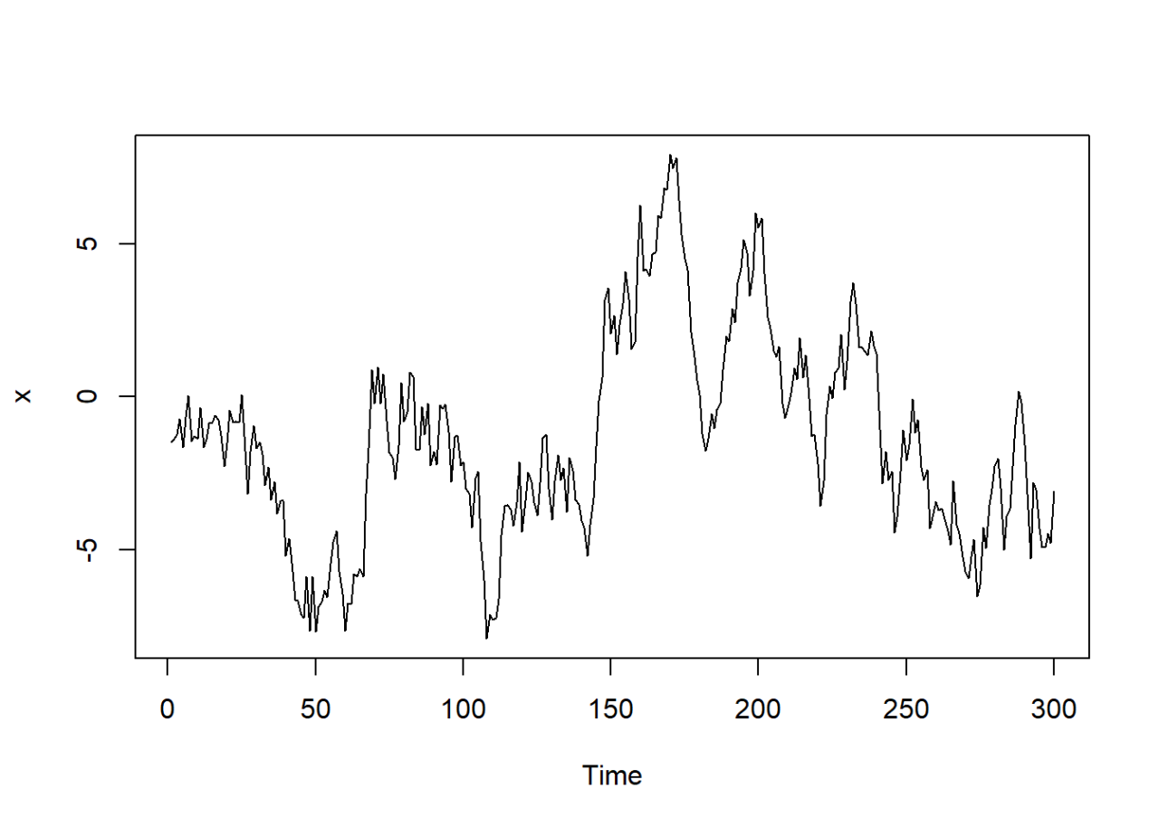
However, if ϕ is very large, say ϕ = 0.95 there is no resemblance to the original white noise sequence.

x = arima.sim(list(ar = .1), n = n, innov = w)
plot.ts(x)

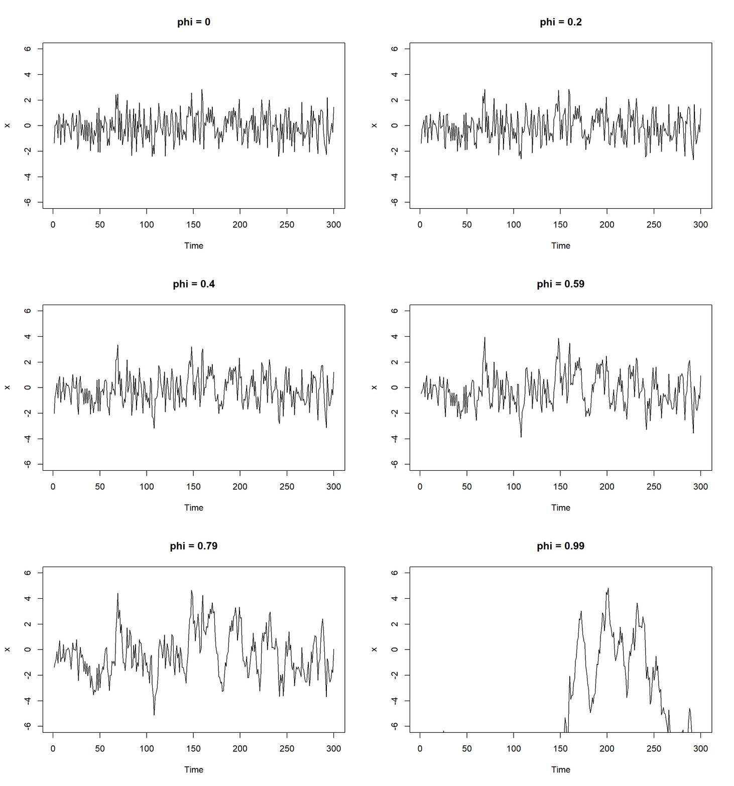
We can animate this movement as we go from ϕ = 0 (white noise) to the boundary ϕ ≈ 1.

phiSeq = seq(0.0001, 0.99, length.out = 100)
plotTitles = paste0("phi = ", as.character(round(phiSeq, 3)))
for(i in 1:100)
{
x = arima.sim(list(ar = phiSeq[i]), n = n, innov = w)
plot.ts(x, ylim = c(-6, 6), main = plotTitles[i])
}

Page Last Revised - December 16, 2022

Is this page helpful?
Thumbs Up Image

Yes

NO THANKS

255 characters maximum

255 characters maximum reached

Thank you for your feedback.
Comments or suggestions?

Top